Numerical Methods for Ordinary Differential Equations (ODEs)

This course covers the fundamentals of solving ordinary differential equations using numerical methods, including Taylor series, Runge Kutta, midpoint, and Heuns methods, as well as techniques for solving systems of ODEs and boundary value problems.
- Uploaded on | 1 Views
-
 abbypollich
About Numerical Methods for Ordinary Differential Equations (ODEs)
PowerPoint presentation about 'Numerical Methods for Ordinary Differential Equations (ODEs)'. This presentation describes the topic on This course covers the fundamentals of solving ordinary differential equations using numerical methods, including Taylor series, Runge Kutta, midpoint, and Heuns methods, as well as techniques for solving systems of ODEs and boundary value problems.. The key topics included in this slideshow are CISE301, SE301, KFUPM, ODEs, numerical methods, Taylor series, Runge Kutta, midpoint method, Heuns method, boundary value problems, systems of ODEs,. Download this presentation absolutely free.
Presentation Transcript
1. CISE301_Topic8L8&9 KFUPM 1 SE301: Numerical Methods Topic 8 Ordinary Differential Equations (ODEs) Lecture 28-36 KFUPM Read 25.1-25.4, 26-2, 27-1
2. CISE301_Topic8L8&9 KFUPM 2 Outline of Topic 8 Lesson 1: Introduction to ODEs Lesson 2: Taylor series methods Lesson 3: Midpoint and Heuns method Lessons 4-5: Runge-Kutta methods Lesson 6: Solving systems of ODEs Lesson 7: Multiple step Methods Lesson 8-9: Boundary value Problems
3. CISE301_Topic8L8&9 KFUPM 3 L ecture 35 Lesson 8: Boundary Value Problems
4. CISE301_Topic8L8&9 KFUPM 4 Outlines of Lesson 8 Boundary Value Problem Shooting Method Examples
5. CISE301_Topic8L8&9 KFUPM 5 Learning Objectives of Lesson 8 Grasp the difference between initial value problems and boundary value problems. Appreciate the difficulties involved in solving the boundary value problems. Grasp the concept of the shooting method. Use the shooting method to solve boundary value problems.
6. CISE301_Topic8L8&9 KFUPM 6 Boundary-Value and Initial Value Problems Boundary-Value Problems The auxiliary conditions are not at one point of the independent variable More difficult to solve than initial value problem Initial-Value Problems The auxiliary conditions are at one point of the independent variable same different
7. CISE301_Topic8L8&9 KFUPM 7 Shooting Method
8. CISE301_Topic8L8&9 KFUPM 8 The Shooting Method Target
9. CISE301_Topic8L8&9 KFUPM 9 The Shooting Method Target
10. CISE301_Topic8L8&9 KFUPM 10 The Shooting Method Target
11. CISE301_Topic8L8&9 KFUPM 11 Solution of Boundary-Value Problems Shooting Method for Boundary-Value Problems 1. Guess a value for the auxiliary conditions at one point of time. 2. Solve the initial value problem using Euler, Runge-Kutta, 3. Check if the boundary conditions are satisfied, otherwise modify the guess and resolve the problem. Use interpolation in updating the guess. It is an iterative procedure and can be efficient in solving the BVP.
12. CISE301_Topic8L8&9 KFUPM 12 Solution of Boundary-Value Problems Shooting Method Boundary-Value Problem Initial-value Problem convert 1. Convert the ODE to a system of first order ODEs. 2. Guess the initial conditions that are not available. 3. Solve the Initial-value problem. 4. Check if the known boundary conditions are satisfied. 5. If needed modify the guess and resolve the problem again.
13. CISE301_Topic8L8&9 KFUPM 13 Example 1 Original BVP 0 1 x
14. CISE301_Topic8L8&9 KFUPM 14 Example 1 Original BVP 2. 0 0 1 x
15. CISE301_Topic8L8&9 KFUPM 15 Example 1 Original BVP 2. 0 0 1 x
16. CISE301_Topic8L8&9 KFUPM 16 Example 1 Original BVP to be determined 2. 0 0 1 x
17. CISE301_Topic8L8&9 KFUPM 17 Example 1 Step1: Convert to a System of First Order ODEs
18. CISE301_Topic8L8&9 KFUPM 18 Example 1 Guess # 1 -0.7688 0 1 x
19. CISE301_Topic8L8&9 KFUPM 19 Example 1 Guess # 2 0.99 0 1 x
20. CISE301_Topic8L8&9 KFUPM 20 Example 1 Interpolation for Guess # 3 Guess y(1) 1 0 -0.7688 2 1 0.9900 0.99 0 1 2 y(0) -0.7688 y(1)
21. CISE301_Topic8L8&9 KFUPM 21 Example 1 Interpolation for Guess # 3 Guess y(1) 1 0 -0.7688 2 1 0.9900 0.99 0 1 2 y(0) -0.7688 1.5743 2 y(1) Guess 3
22. CISE301_Topic8L8&9 KFUPM 22 Example 1 Guess # 3 2.000 0 1 x This is the solution to the boundary value problem. y(1)=2.000
23. CISE301_Topic8L8&9 KFUPM 23 Summary of the Shooting Method 1. Guess the unavailable values for the auxiliary conditions at one point of the independent variable. 2. Solve the initial value problem. 3. Check if the boundary conditions are satisfied, otherwise modify the guess and resolve the problem. 4. Repeat (3) until the boundary conditions are satisfied.
24. CISE301_Topic8L8&9 KFUPM 24 Properties of the Shooting Method 1. Using interpolation to update the guess often results in few iterations before reaching the solution. 2. The method can be cumbersome for high order BVP because of the need to guess the initial condition for more than one variable.
25. CISE301_Topic8L8&9 KFUPM 25 L ecture 36 Lesson 9: Discretization Method
26. CISE301_Topic8L8&9 KFUPM 26 Outlines of Lesson 9 Discretization Method Finite Difference Methods for Solving Boundary Value Problems Examples
27. CISE301_Topic8L8&9 KFUPM 27 Learning Objectives of Lesson 9 Use the finite difference method to solve BVP. Convert linear second order boundary value problems into linear algebraic equations.
28. CISE301_Topic8L8&9 KFUPM 28 Solution of Boundary-Value Problems Finite Difference Method y 4 =0.8 0 0.25 0.5 0.75 1.0 x x0 x1 x2 x3 x4 y y 0 =0.2 y 1 =? y 2 =? y 3 =? Boundary-Value Problems Algebraic Equations convert Find the unknowns y 1 , y 2 , y 3
29. CISE301_Topic8L8&9 KFUPM 29 Solution of Boundary-Value Problems Finite Difference Method Divide the interval into n intervals. The solution of the BVP is converted to the problem of determining the value of function at the base points. Use finite approximations to replace the derivatives. This approximation results in a set of algebraic equations. Solve the equations to obtain the solution of the BVP.
30. CISE301_Topic8L8&9 KFUPM 30 Finite Difference Method Example y 4 =0.8 0 0.25 0.5 0.75 1.0 x x0 x1 x2 x3 x4 y y 0 =0.2 Divide the interval [0,1 ] into n = 4 intervals Base points are x0=0 x1=0.25 x2=.5 x3=0.75 x4=1.0 y1=? y2=? y3=? To be determined
31. CISE301_Topic8L8&9 KFUPM 31 Finite Difference Method Example Divide the interval [0,1 ] into n = 4 intervals Base points are x0=0 x1=0.25 x2=.5 x3=0.75 x4=1.0
32. CISE301_Topic8L8&9 KFUPM 32 Second Order BVP
33. CISE301_Topic8L8&9 KFUPM 33 Second Order BVP
34. CISE301_Topic8L8&9 KFUPM 34 Second Order BVP
35. CISE301_Topic8L8&9 KFUPM 35 Second Order BVP
36. CISE301_Topic8L8&9 KFUPM 36
37. CISE301_Topic8L8&9 KFUPM 37 Summary of the Discretiztion Methods Select the base points. Divide the interval into n intervals. Use finite approximations to replace the derivatives. This approximation results in a set of algebraic equations. Solve the equations to obtain the solution of the BVP.
38. CISE301_Topic8L8&9 KFUPM 38 Remarks Finite Difference Method : Different formulas can be used for approximating the derivatives. Different formulas lead to different solutions. All of them are approximate solutions. For linear second order cases, this reduces to tri-diagonal system.
39. CISE301_Topic8L8&9 KFUPM 39 Summary of Topic 8 Solution of ODEs Lessons 1-3: Introduction to ODE, Euler Method, Taylor Series methods, Midpoint, Heuns Predictor corrector methods Lessons 4-5: Runge-Kutta Methods (concept & derivation) Applications of Runge-Kutta Methods To solve first order ODE Lessons 6: Solving Systems of ODE Lessons 8-9: Boundary Value Problems Discretization method Lesson 7: Multi-step methods