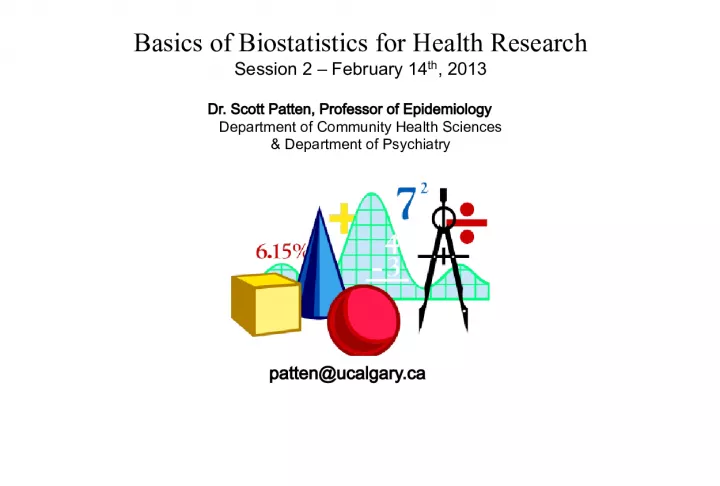
Basics of Biostatistics for Health Research Session 2 with Dr. Scott Patten

Slide1Basics of Biostatistics for Health ResearchSession 2 – February 14 th , 2013 Dr. Scott Patten, Professor of Epidemiology Department of Community Health Sciences & Department of Psychiatry patten@ucalgary.ca

Slide2•Go to “www.ucalgary.ca/~patten” www.ucalgary.ca/~patten • Scroll to the bottom. • Right click to download the files described as being “for PGME Students” – One is a dataset – One is a data dictionary • Save them on your desktop

Slide3Open the Datafile

Slide4The task from last week…• Create a 95% exact binomial confidence interval for the proportion of people with Framingham with > H.S. education

Slide5Review of Last Week’s Task• “use” • “generate” • “recode” • “tabulate” • “ci”

Slide6The actual commands…generate highschool = educ recode highschool 1/2=0 3/4=1 tabulate highschool ci highschool, binomial

Slide7Creating a “do” file…1 2 3

Slide8The “do file” editor

Slide9Executing a “do” file

Slide10What is a “do” file?• It is a text file – you can copy and paste from the output window in Stata, or from a word processor • It is a computer program that consists of actual commands and therefore doesn’t need a compiler • Others would call it a “macro”

Slide11Different Types of Data• One type of distinction – Nominal (e.g. sex, race) – Ordinal (e.g. rating scales) – Cardinal (e.g. physical measures) • Another type of distinction – Categorical (e.g. # of pregnancies) – Continuous (e.g. height, weight)

Slide12Body Mass Index (BMI)

Slide13The BMI in our Data SetThis is an example of a continuous variable

Slide14Changing Data Types in Stata(e.g. continuous to categorical) • recode bmi x/y=z • This will recode all values of the variable bmi having values from x to y to a single value equal to z.

Slide15Interpretation of BMI• Underweight: < 18.5 • Normal weight: 18.5 to 25 • Over weight: >25 to 30 • Obese: 30+ • Your task :  Make a “do file” that calculates a 95% confidence interval for the proportion of the population that are overweight or obese.

Slide16Example of Code for this…generate owo = bmi recode owo 0/25 = 0 25.01/100 = 1 tab owo, missing ci owo, binomial

Slide17Another Task…• Add a use command to your do file • Save your “do file” on the desktop using a descriptive file name of your choice • Exit Stata • Open Stata again • Open the “do file” editor and select your do file • Execute your “do file”

Slide18The Power of “do files”• Task :  Calculate an exact 95% CI for the proportion of the population that are obese (BMI > 30) • IMPORTANT:  do NOT start from scratch as we did before – try to do this by editing your do file.

Slide19generate owo = bmirecode owo 0/25 = 0 25.01/100 = 1 tab owo, missing ci owo, binomial generate owo = bmi generate obese = bmi recode owo 0/25 = 0 25.01/100 = 1 recode obese 0/30 = 0 30.01/100=1 tab owo, missing tab obese, missing ci owo obese, binomial For Example…

Slide20Starting a Log File1 2 3

Slide21Closing a Log File1 2 3

Slide22Another Task…• Start a log file • Run your “do file” • Close and save the resulting log file on your desktop • Open your log file

Slide23“do file” Etiquette• When you add an * before a line on a “do file” Stata will ignore that line • Use this to…. – Add descriptive comments to your code – Remove commands that you don’t want now, but might want later

Slide24E.g. Without the Tables…

Slide25Review…• Make a value label for obesity • Attach this value label to the variable representing obesity

Slide26Making a Graphic

Slide27The Pie Chart Dialogue BoxFind the Variable that you made 1 2

Slide28Unedited Output

Slide29The Graph Editor

Slide30Here is a good place to start

Slide31See if you can do these things…• Change the color of the pie • Add a title • Add a comment • Change the background • Create a work of art

Slide32Save in a Standard Format

Slide33Back to BMI• May not wish to categorize variables like this • Measures of central tendency – Mode – Median – Mean • Different types of graphs are useful for examining continuous variables – Box plots – Histograms

Slide34Box Plots

Slide35Terminology• Median: value with 50% of observations above and 50% below. • Interquartile range – contains 50% of observations – plus or minus one quartile • Adjacent values (whiskers) – observation that is less than 1.5x the IQR • Outliers: anything outside of the adjacent values

Slide36Calculating Summary StatsCalculate summary stats for BMI

Slide37Calculating Summary StatsCalculate the mean BMI

Slide38Calculating Summary StatsCalculate median BMI

Slide39Make a Box (and whisker) Plot

Slide40The Boxplot Dialogue Box1 2 Select BMI from the dropdown list

Slide41Introducing Histograms1 2

Slide42The Histogram Dialogue BoxSelect the variable here Select the bin# here

Slide43A Task for You to Do…• Make 3 histograms of BMI – In one use the default number of bins – In one use a larger number – In one, use a smaller number • Save your favorite histogram • Open it in the graph editor, give it a title and improve its appearance • Save it in a standard form (e.g. png, jpg, tif)

Slide44Assessing Normality with a Histogram

Slide45The distribution is not quitenormal, but close

Slide46Is BMI Higher in Men orWomen? • We could use confidence intervals to assess this… • E.g. 1 2 3

Slide47Here is the dialogue box…Once you’ve selected BMI, click this

Slide48The dialogue box, continued..Enter sex as a group variable

Slide49The output

Slide50It looks better with value labels

Slide51Statistical Tests• Start with an hypothesis that an “effect” exists – In this case, that there is an effect of sex on BMI • Assume that the effect DOES NOT exist – This is the null hypothesis • Find the probability of results, or those more extreme given the null hypothesis – This is what the “test” calculates for you • If the null is unlikely (alpha value), reject it

Slide52The t-test (assumptions)• The variables are approximately normally distributed • The standard deviations of the two groups are approximately equal • The two samples are independent

Slide53Using summarize  similarly • Use  summarize  with “ by ” in the dialogue box • Use  histograms  with a normal density plot and the “ by ” tab in the dialogue box Your task:  use these two techniques to assess the t-test assumptions.

Slide54Variance Comparisons1 2 3

Slide55The t-test1 2 3

Slide56The t-test dialogue box1 2 3 optional

Slide57The output

Slide58Two group tests for proportions..1 3 2

Slide59You can also do this with tab tab obese sex, exact

Slide60Your Final Task for Today• Create a “do file” that … – Reads in the data – Recodes BMI to a categorical variable for obesity – Tests whether obesity differs between men and women • Create a log file to store the results