Limited Dependent Variables in Economics

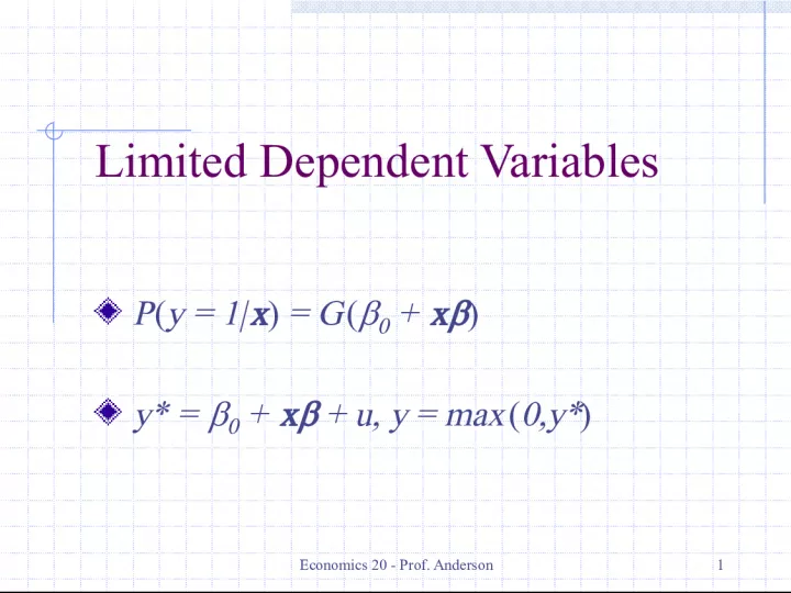
1. Economics 20 - Prof. Anderson 1 Limited Dependent Variables P ( y = 1| x ) = G ( 0 + x ) y* = 0 + x + u, y = max ( 0,y* )

2. Economics 20 - Prof. Anderson 2 Binary Dependent Variables Recall the linear probability model, which can be written as P( y = 1| x ) = 0 + x A drawback to the linear probability model is that predicted values are not constrained to be between 0 and 1 An alternative is to model the probability as a function, G ( 0 + x ), where 0< G ( z )<1

3. Economics 20 - Prof. Anderson 3 The Probit Model One choice for G ( z ) is the standard normal cumulative distribution function (cdf) G ( z ) = ( z ) ( v )d v , where ( z ) is the standard normal, so ( z ) = (2 ) -1/2 exp(- z 2 /2) This case is referred to as a probit model Since it is a nonlinear model, it cannot be estimated by our usual methods Use maximum likelihood estimation

4. Economics 20 - Prof. Anderson 4 The Logit Model Another common choice for G(z) is the logistic function, which is the cdf for a standard logistic random variable G ( z ) = exp( z )/[1 + exp( z )] = ( z ) This case is referred to as a logit model, or sometimes as a logistic regression Both functions have similar shapes they are increasing in z , most quickly around 0

5. Economics 20 - Prof. Anderson 5 Probits and Logits Both the probit and logit are nonlinear and require maximum likelihood estimation No real reason to prefer one over the other Traditionally saw more of the logit, mainly because the logistic function leads to a more easily computed model Today, probit is easy to compute with standard packages, so more popular

6. Economics 20 - Prof. Anderson 6 Interpretation of Probits and Logits (in particular vs LPM) In general we care about the effect of x on P( y = 1 | x ), that is, we care about p / x For the linear case, this is easily computed as the coefficient on x For the nonlinear probit and logit models, its more complicated: p / x j = g ( 0 + x ) j , where g ( z ) is d G /d z

7. Economics 20 - Prof. Anderson 7 Interpretation (continued) Clear that its incorrect to just compare the coefficients across the three models Can compare sign and significance (based on a standard t test) of coefficients, though To compare the magnitude of effects, need to calculate the derivatives, say at the means Stata will do this for you in the probit case

8. Economics 20 - Prof. Anderson 8 The Likelihood Ratio Test Unlike the LPM, where we can compute F statistics or LM statistics to test exclusion restrictions, we need a new type of test Maximum likelihood estimation (MLE), will always produce a log-likelihood, L Just as in an F test, you estimate the restricted and unrestricted model, then form LR = 2( L ur L r ) ~ 2 q

9. Economics 20 - Prof. Anderson 9 Goodness of Fit Unlike the LPM, where we can compute an R 2 to judge goodness of fit, we need new measures of goodness of fit One possibility is a pseudo R 2 based on the log likelihood and defined as 1 L ur / L r Can also look at the percent correctly predicted if predict a probability >.5 then that matches y = 1 and vice versa

10. Economics 20 - Prof. Anderson 10 Latent Variables Sometimes binary dependent variable models are motivated through a latent variables model The idea is that there is an underlying variable y*, that can be modeled as y * = 0 + x + e , but we only observe y = 1, if y * > 0, and y =0 if y * 0,

11. Economics 20 - Prof. Anderson 11 The Tobit Model Can also have latent variable models that dont involve binary dependent variables Say y * = x + u , u| x ~ Normal(0, 2 ) But we only observe y = max(0, y *) The Tobit model uses MLE to estimate both and for this model Important to realize that estimates the effect of x on y*, the latent variable, not y

12. Economics 20 - Prof. Anderson 12 Interpretation of the Tobit Model Unless the latent variable y * is whats of interest, cant just interpret the coefficient E( y| x ) = ( x / ) x + x / , so E( y| x ) / x j = j ( x / ) If normality or homoskedasticity fail to hold, the Tobit model may be meaningless If the effect of x on P( y >0) and E( y ) are of opposite signs, the Tobit is inappropriate

13. Economics 20 - Prof. Anderson 13 Censored Regression Models & Truncated Regression Models More general latent variable models can also be estimated, say y = x + u , u| x ,c ~ Normal(0, 2 ), but we only observe w = min( y,c ) if right censored, or w = max(y,c) if left censored Truncated regression occurs when rather than being censored, the data is missing beyond a censoring point

14. Economics 20 - Prof. Anderson 14 Sample Selection Corrections If a sample is truncated in a nonrandom way, then OLS suffers from selection bias Can think of as being like omitted variable bias, where whats omitted is how were selected into the sample, so E( y|z , s = 1) = x + ( z ), where ( c ) is the inverse Mills ratio: ( c )/ ( c )

15. Economics 20 - Prof. Anderson 15 Selection Correction (continued) We need an estimate of , so estimate a probit of s (whether y is observed) on z These estimates of can then be used along with z to form the inverse Mills ratio Then you can just regress y on x and the estimated to get consistent estimates of Important that x be a subset of z , otherwise will only be identified by functional form