1. Fundamentals of Statistics: Examples and Explanations This presentation provides a detailed explanation of statistical concepts and uses examples from a renowned textbook.

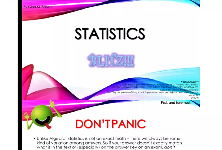
1. STATISTICS STATISTICS By Gina M. Salvati *~DISCLAIMER~* Some examples are lifted from Fundamentals of Statistics Third Edition. All rights reserved, yada, yada, yada. I dont own those examples, and they are noted throughout the presentation. The only people benefitting from this presentation (hopefully) are peer tutors and the students. ENJOY!

2. DONT PANIC DONT PANIC Unlike Algebra, Statistics is not an exact math there will always be some kind of variation among answers. So if your answer doesnt exactly match what is in the text or (especially) on the answer key on an exam, dont panic . As long as you are in the same ballpark as the given answer(s), you should be just fine. Even with that being said, however, always, always, always check your work. It is always important to double-check yourself, no matter which course you take. A good test-taking tip when it comes to multiple choice is to go with the answer closest to what you come up with. First, and foremost

3. THE CHAMBER OF DOOM (I Mean, Table of Contents )

4. THE TYPES OF CURVES Right-skew Right-skew Symmetrical Symmetrical AKA AKA Bell Curve Bell Curve Left-skew Left-skew In the image above, the relationships of mean, median, and mode are illustrated. Mean < Median < Mode Mean < Median < Mode Mean > Median > Mode Mean > Median > Mode Mean = Median = Mode Mean = Median = Mode

5. MEASURES OF CENTRAL TENDENCY VS. MEASURES OF DISPERSION

6. MEASURES OF CENTRAL TENDENCY VS. MEASURES OF DISPERSION

7. HOW TO CALCULATE ON TI-83/84 From Fundamentals of Statistics Third Edition text, pg. 125.

8. Z-SCORES Lets see an example

9. Z-SCORES From Fundamentals of Statistics Third Edition text, pg. 161.

10. THE FIVE-NUMBER SUMMARY, BOXPLOTS, AND OUTLIERS

11. TO CONSTRUCT A BOXPLOT After entering your data in L 1 , hit 2 nd , Y=. This will bring you to the Stat Plots screen. Hit ENTER or 1. This will bring you to another screen, where you can actually set up the boxplot. Turn the plots ON. Select the Boxplot with Outliers type. This is the first image in the second row in the Types category. Zoom, 9: ZoomStat Ta-da! :D

12. THE INTERQUARTILE RANGE

13. TO DETERMINE OUTLIERS

14. THE FIVE-NUMBER SUMMARY, BOXPLOTS, AND OUTLIERS April Showers The following data represent the number of inches of rain in Chicago, Illinois, during the month of April for 20 randomly selected years. [a] Determine the five-number summary [b] Compute the Interquartile Range (IQR) [c] Determine the Upper and Lower Fences. Are there any outliers? EXAMPLE TIME! 0.97 2.47 3.94 4.11 5.79 1.14 2.78 3.97 4.77 6.14 1.85 3.41 4.00 5.22 6.28 2.34 2.34 4.02 5.50 7.69 Fundamentals of Statistics Third Edition , pg. 162

15. THE FIVE-NUMBER SUMMARY, BOXPLOTS, AND OUTLIERS ANSWERS

16. LINEAR REGRESSION AND WHAT ALL GOES WITH IT What is r and r 2 ? Well, lets take a look Look at this equation setup here. It should look familiar. (Hint: substitute m for a )

17. R AND R 2 The linear correlation coefficient (r) measures how closely related the data is to the linear regression line The coefficient of determination (r 2 ) holds explaining power: the linear regression explains __ much of the data. Note: It is important to remember that correlation doesnt necessarily imply causation just because there is a correlation between two variables, it doesnt always mean that one is causing the other.

18. A QUICK LOOK AT PROBABILITY

19. THE EMPIRICAL RULE The Empirical Rule is used to give us an approximation of the number(s) that lies within 1, 2, or 3 standard deviations away from the mean. 68% of the distribution lies within 1 deviation from the mean 95% of the distribution lies within 2 deviations of the mean 99.7% of the distribution lies within 3 deviations of the mean

20. THE EMPIRICAL RULE: A SLIGHTLY BETTER EXAMPLE 68% 100 + 5 = 105 100 5 = 95 95% 99.7% 105 + 5 = 110 95 5 = 90 110 + 5 = 115 90 5 = 85

21. WHAT TO USE AND WHEN TO USE IT {PT. 1}: NORMALCDF VS. INVNORM Two simple calculator functions that can very easily get mixed up. These are the key things to remember about normalcdf and invNorm: normalcdf: When were given z-scores or data points* and asked to find the probability/proportion/area under the curve. invNorm: When were given a percent/probability/area and asked to find the z-score/data point . A trick is to look for key words. One example is the word percentile . If a question asks you to find a percentile, you will use the invNorm function on your calculator.

22. NORMALCDF ON THE CALCULATOR When using the normalcdf function on your calculator, the order of input is the lower bound, followed by the upper bound, then the mean, and finally the standard deviation. Most calculators will have you enter the information manually; others are kind enough to help you out a little: -E99 and E99 are very useful in circumstances when you are not given an upper or lower bound. In some instance, -100 and 100 can be used, but sometimes a much smaller or larger may be called for. To put this in the calculator, press 2 nd and then the comma key to get E. Simply type the negative symbol before if doing E99.

23. NORMALCDF EXAMPLE If I were to ask what the area under the curve was above 1.50, my graph would look something like this: If were to ask what the area under the curve was below 1.50, my graph would look like this: And if I wanted to know the area between , say, -1.75 and 1.5, my graph would look like this: NOTE: In this example, we are working with the standard normal curve . This means that = 0 and = 1.

24. INVNORM ON THE CALCULATOR When using the invNorm function on your calculator, the order of input is the area to the left of the z-score were seeking, followed by the mean, and finally the standard deviation. Most calculators will have you enter the information manually; others are kind enough to help you out a little:

25. INVNORM EXAMPLE 1.0 invNorm problems can get a little confusing at times. The key, as with virtually everything in Statistics, is in the wording. Lets say I am in charge of a chocolate chip cookie factory. The factory churns out an average of 3500 cookies a day, with a standard deviation of 45. Inventory is just around the corner, and were expected to make above the 60 th percentile. Over how many cookies are we supposed to make to meet expectations? The wording here isnt exactly the greatest, but we are given the information necessary to perform the task. We know that we a have an average (mean, ) of 3500 cookies and a standard deviation ( ) of 45. We also know that we need to make above the 60 th percentile. This means we need to make over the first 60% in order to meet the quota. How do we solve for this?

26. INVNORM EXAMPLE 1.0 (CONT.) The easiest way to solve is to start out by drawing a picture: The 60 th percentile is illustrated as the first 60% of our distribution. Using some more of our newly discovered mad calculator skills, we can find the number of cookies (our data point) by following these steps: 2 nd , vars, 3: invNorm Enter, in order, the area to the left side of the data point we are seeking (here, .60), the mean, and the standard deviation ENTER The number you get will be the data point were looking for. The answer here comes out to be 3511.40062. Because we are talking about cookies and not random numbers, it is best to round. A good practice is to round up, to take into account for potential extra. ANSWER: In order to meet expectations, the factory needs to make over 3511/3512 cookies.

28. THE SAMPLING DISTRIBUTION OF THE SAMPLE MEAN Lets see an example This cute little equation is called the standard error of the mean , or just standard error . Good little vocab hint to remember. ;)

29. From Fundamentals of Statistics, Third Edition, pg. 389

30. EXAMPLE PROBLEM #1 SOLUTION

31. EXAMPLE PROBLEM #1 SOLUTION (CONT.) Please note: images arent exactly to scale. ^^;;

32. THE SAMPLING DISTRIBUTION OF THE POPULATION PROPORTION This equation is for a point estimate. We use this to adjust our numbers in order to fit the distribution. If youre dealing with decimals, a whole number isnt going to fall in your distribution. ;)

33. Smith owns a shipyard. He knows that 5% of all welding done that afternoon will wind up being defective. Out of the 7000 welds in the yard, he examines 300. Whats the probability that between 10 and 20 welding jobs will be defective?

34. SMITH AND HIS SHIPYARD

35. SMITH AND HIS SHIPYARD (CONT.)

36. WHAT TO USE AND WHEN TO USE IT {PT. 2}: CONFIDENCE INTERVALS Stat, Tests, 7: Z-Int when given (population standard deviation) 8: T-Int when given s (sample standard deviation) or no standard deviation when given a data set A: 1-PropZInt when given x and n values (a sample, n, and a number out the sample, x) and a percent or proportion B: 2-PropZInt when given two x and n values (two samples and numbers out of those samples: x 1 and n 1, and x 2 and n 2 ) A Quick Run-Down

37. WHAT TO USE AND WHEN TO USE IT {PT. 3}: THE INSANITY THAT IS HYPOTHESIS TESTING Stat, Tests, 1: Z-Test when given (population standard deviation) 2: T-Test when given s (sample standard deviation) or no standard deviation when given a data set 5: 1-PropZTest when given x and n values (a sample, n, and a number out of the sample, x) and a percent or proportion 6: 2-PropZTest when given two x and n values (two samples and numbers out of those samples: x 1 and n 1, and x 2 and n 2 ) A Quick Run-Down

38. FEAT. TYPE I AND TYPE II ERRORS The best way to describe these two is to think about hypothesis testing as a court case. The old motto of innocent until proven guilty provides us with our null and alternative hypotheses. The following is a mini-cartoon illustrating Type I and Type II errors.

40. WHAT TO USE AND WHEN TO USE IT {THE FINALE}: MATCHED-PAIR DATA VS. CHI-SQUARE GOF TESTING Now, this is where things are confusing. Because these two types of testing appear so alike when entering data into the calculator, its easy to get confused. How can we tell the difference between these two kinds of problems??? WHAT TO LOOK FOR, HOW TO SOLVE The problems from these two sections appear to be very similar, but they are very different . Its important to remember when to use either method of solving. Lets take a look at a couple of examples

41. MATCHED-PAIR DATA On one final exam study guide, there is a problem that talks about a football coach claiming that players can increase their strength by taking a certain supplement. He decides to test this theory by randomly selecting 9 athletes and gives them a strength test on the bench press. 30 days later, after regular training and taking this supplement, he tests them again. First of all, we need to identify what kind of problem this is. I just identified it as a matched-pair data problem. How can you tell if its this and not chi-square goodness- of-fit? Look at the data table: We want to test if the coachs claim holds that the supplement is effective in increasing the athletes strength. Athlete 1 2 3 4 5 6 7 8 9 Before 215 240 188 212 275 260 225 200 185 After 225 245 188 210 282 275 230 195 190

42. MATCHED-PAIR DATA The Before values are the first set of data we gathered. These will go into List 1 (Stat, Edit, 1). The values in the second data set we gathered (After) will go into List 2. Okay, now we need to see how the difference between these two data sets levels out in our test against our level of significance, = 0.05. To do this, we first need to get the differences, and we do that by highlighting the List 3 heading and entering the equation L 1 L 2 and pressing the ENTER key. This will give you a list of numbers the difference between List 1 and List 2. Exit the screen by pressing 2 nd , mode. Then, go to Stat, Tests, 2 (Z-Test), and use the DATA option for your input. Change the List selection from L 1 to L 3 , and proceed accordingly with your hypothesis testing. In short: L 1 before values L 2 after values L 3 heading L 1 L 2 2 nd , mode (to get out) Stat, Tests, 2 (Z-Test) Data Look at L 3 **Note**: When writing out your null and alternate hypotheses, remember the H 0 will always be = 0, to indicate that there is no difference in values. To determine H 1 , look at the alternative claim.

43. Remember: Problems from Matched-Pair Data and Chi-Square may look somewhat similar, but they are very different . The confusion lies in 1.) identifying the problem and 2.) remembering which equation to put in the L 3 heading. * *If you have a TI-84 calculator, there is a trick to avoid this issue. The trick will be covered in another slide.

44. CHI-SQUARE Again, problems from this section and from matched-pair data may look somewhat similar, but they are very different . Here is an example: The information provided in one problem from a former exam review gives us the number of wins for track hurdlers and asks us to test the claim that the probabilities of winning are the same in different positions. Again, we have to identify whether this is actually chi-square and not matched-pair data. Look at the chart, which Ive added to here as well: Unlike the previous question, which gave us before and after values, this gives us a table of observed outcomes. This is where we can tell what the difference is: matched-pair data are generally given as before and after, whereas chi-square gives us an expectation and what we actually observed happening. Now that we know this much, what is our expectation for this equation? Like any other hypothesis test, we have to identify a null hypothesis and an alternative hypothesis. In this case, our null is what we expected. For a problem like this, we would expect that, if a runner each lane had equal chances of winning, each lane would get a 1/6 chance. Starting Position 1 2 3 4 5 6 Number of Wins 45 50 36 44 32 33

45. CHI-SQUARE (CONT) How does this work on a calculator? Similar to matched-pair data problems, we start out by entering data (Stat, Edit, 1). In L 1 , we put our observed data what actually happened. This would be the number of wins represented in the table above. In L 2 , we take the total number of wins (here, 240) and multiply it by the chance we expected (1/6). And in the L 3 heading, we use the equation (L 1 L 2 ) 2 /L 2 . In short: L 1 observed outcomes (what really happened); number of wins in graph L 2 expected outcomes (what we thought was going to happen); total wins * chance of winning (250 * 1/6) L 3 heading (L 1 L 2 ) 2 /L 2 2 nd , mode (to get out) 2 nd , Stat, < , Math, 5 (sum) Find the sum of L 3 This is your test statistic Proceed accordingly with hypothesis testing

46. CHI-SQUARE (CONT.) (PLEASE NOTE: this trick only works on TI-84 calculators; TI-83 calculators do not have this function!)

47. YOU AINT NEVER HAD A FRIEND LIKE... Given Hypothesis Testing Confidence Intervals (population standard deviation) 1 7 s (sample standard deviation) or no standard deviation when given a data set 2 8 When given x and n values (a sample, n, and a number out of the sample, x) 5 A When given x and n values for two samples (x 1 and n 1 , x 2 and n 2 ) 6 B The Ultimate Wrap-Up for What to Use and When to Use it! :D

48. THE END! This concludes the Statistics Blitz PowerPoint Presentation Created by Gina M. Salvati, CRLA certified tutor and former peer tutor for North Florida Community College and Florida Gateway College Version updated: 2014.9.15