Chapter 2 - Central Tendency & Variability

This chapter covers measures of central tendency, which are used to determine a typical or average value in a set of data. The Mean, which is the sum of all scores divided
- Uploaded on | 1 Views
-
 kari
kari
About Chapter 2 - Central Tendency & Variability
PowerPoint presentation about 'Chapter 2 - Central Tendency & Variability'. This presentation describes the topic on This chapter covers measures of central tendency, which are used to determine a typical or average value in a set of data. The Mean, which is the sum of all scores divided. The key topics included in this slideshow are . Download this presentation absolutely free.
Presentation Transcript
Slide1Chapter 2Central Tendency & Variability Tues. Aug. 27, 2013
Slide2Measures of Central Tendency TheMean • Sum of all the scores divided by the number of scores • Mean of 7,8,8,7,3,1,6,9,3,8 – Σ X = – N = 10 – Mean (or M) =
Slide3The Mode• Most common single number in a distribution • Mode of 7,8,8,7,3,1,6,9,3,8? • Measure of central tendency for nominal variables (most common category was…)
Slide4The Median• The middle score when all scores are arranged from lowest to highest • Median of 7,8,8,7,3,1,6,9,3,8 – 1 3 3 6 7 7 8 8 8 9 median – Median is the average (mean) of the 5 th and 6 th scores here – ? How do we decide between using mean or median?
Slide5The Median• With large data sets, shortcut… – If odd N, divide by 2, then add ½, gives position of the median score in list. • Ex? – If even N, divide by 2, this and score above it need to be averaged for median. • ex?
Slide6Example of Mean/Median Preference• Evolutionary psych example in book (p. 40-41) – competing theories of gender diffs in how many mates we prefer – Buss (evol.) – men should prefer more partners than women (to spread genes) – Miller – men/women should prefer same #
Slide7•Table 2-1, data from 106 men, 160 women • Women’s M=2.8, Median = 1, Mode = 1 • Men’s M=64.3, Median = 1, Mode = 1 • See Fig 2-8, how do outliers affect the mean in this study? Median?
Slide8Location of Mean, Mode, Median
Slide9Measures of SpreadThe Variance • The average of each score’s squared difference from the mean • Steps for computing the variance: 1. Subtract the mean from each score 2. Square each of these deviation scores 3. Add up the squared deviation scores 4. Divide the sum of squared deviation scores by the number of scores
Slide10Measures of SpreadThe Variance • Formula for the variance: SD=Standard Deviation (when squared = variance) SS- Sum of Squares
Slide11What variance tells us• Conceptually, it is the average of the squared deviation scores, so… – The more spread out the distribution, the larger the variance • What if variance = 0? – Very important for many stat tests – Conceptual difference in unit of variance versus standard deviation? • Which is more intuitive?
Slide12Measures of SpreadThe Standard Deviation • Most common way of describing the spread of a group of scores • Steps for computing the standard deviation: 1. Figure the variance 2. Take the square root • Conceptually, it is the average of deviations from the mean. – How much do most scores differ from the mean?
Slide13Measures of SpreadThe Standard Deviation • Formula for the standard deviation:
Slide14SD Computational Formula:• Easier to use w/large data sets • Uses sum of x scores ( X ) and sum of squared x scores ( X 2 ) • SD 2 = X 2 – [ ( X) 2 / N] N • Note that your book prefers the definitional formula, not this one • p. 51 – some instances when we divide SS by N-1