Understanding Linear Integer Programming and its Applications

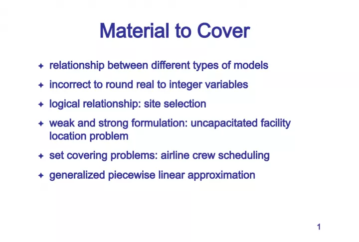
1. 1 Material to Cover relationship between different types of models incorrect to round real to integer variables logical relationship: site selection weak and strong formulation: uncapacitated facility location problem set covering problems: airline crew scheduling generalized piecewise linear approximation

2. 2 max/min z = c 1 x 1 + c 2 x 2 + + c n x n s . t . a i 1 x 1 + a i 2 x 2 + + a in x n b i , i = 1,, m 0 x j u j , j = 1,, n x j integer for some or all j =1,, n { } Linear Integer Programming - IP

3. 3 mixed IP (MIP): some x j Z #1 , some x j # 2 pure IP: all x j Z binary decision variable : x j = 1 or 0 (e.g., a variable for a yes-no decision) binary IP (BIP): all x j being binary Linear Integer Programming - IP #1 Z: the set of integers; Z + : the set of positive integers #2 : the set of real numbers ; + : the set of positive real numbers

4. 4 Motivation of Studying IP integer variables in some context e.g., machine, manpower logical relationship incorrect to round continuous variables

5. 5 Incorrect to Round Continuous Variables optimal LP solution X 1 X 2 optimal IP solution iso-cost line usually all right to round in real life problems with large x i

6. 6 Example to Motivate IP site selection: three designs A , B , C on sites 1, 2, 3, 4 total amount for investment: $100 M how to invest? Option A 1 A 2 A 3 A 4 B 1 B 2 B 3 B 4 C 1 C 2 C 3 C 4 Net Income ($M) 6 7 9 11 12 15 5 8 12 16 19 20 Investment ($M) 13 20 24 30 39 45 12 20 30 44 48 55

7. 7 Example to Motivate IP I = { A , B , C , D }, J = {1, 2, 3, 4} y ij = 1 iff design i used at site j , i I, j J max z = i I p ij y ij s . t . i I j J a ij y ij 100 y ij {0, 1}, i I , j J optimal solution: y A 1 = y A 3 = y B 3 = y B 4 = y C 1 = 1; z * = 40

8. 8 Example to Motivate IP boss says NO! at most one design at a site a building at site 2 (required) at most two designs at the three sites design A considered for sites 1, 2, and 3 only if being used at site 4 how to model?

9. 9 Example to Motivate IP at most one design at a site and a building at site 2 (required) y A 1 + y B 1 + y C 1 1, y A 2 + y B 2 + y C 2 = 1, y A 3 + y B 3 + y C 3 1, y A 4 + y B 4 + y C 4 1 design A considered for sites 1, 2, and 3 only if being used at site 4 y A 1 + y A 2 + y A 3 3 y A 4

10. 10 Example to Motivate IP at most two designs at the three sites w i = 1, if design i is used, = 0, o.w . , i = A , B , C w A + w B + w C 2 y i 1 + y i 2 + y i 3 + y i 4 4 w i , i = A , B , C optimal solution: y A 1 = y A 4 = y B 2 = y B 3 = 1; others = 0; z * = 37

11. 11 Logical Constraints for Variables n situations how to model (i) at most k of them hold, (ii) at least k of them hold, and (iii) exactly k hold y j binary variables for j = 1 to n; y j = 1 if j holds, and = 0 otherwise mutually exclusive y j : y 1 + y 2 + + y n 1 at most k of y j = 1: y 1 + y 2 + + y n k at least k of y j = 1: y 1 + y 2 + + y n k exactly k of y j = 1: y 1 + y 2 + + y n = k

12. 12 Logical Constraints for Expressions either-or constraints either f 1 ( x 1 , , x n ) b 1 or f 2 ( x 1 , , x n ) b 2 or both IP formulation: let y be a binary variable M : a large positive number, practically two constraints: f 1 ( x 1 , , x n ) b 1 + My and f 2 ( x 1 , , x n ) b 2 + M (1- y ) only one of these two being picked by the optimization procedure

13. 13 Logical Constraints for Expressions m constraints, at least k out of m being true f 1 ( x 1 , , x n ) b 1 , , f m ( x 1 , , x n ) b m modeling procedure m binary variables y i , one for each constraint f 1 ( x 1 , , x n ) b 1 + M (1- y 1 ), , f m ( x 1 , , x n ) b m + M (1- y m ) y 1 + + y m k

14. 14 An Example of Logical Constraints for Expressions single processor for three jobs, of processing times 3 hr, 5 hr, and 7 hr, respectively objective: minimizing the total completion time of the three jobs how to formulate it as an integer program? note . The IP is for the illustration of formulation. The problem has very simple solution.

15. 15 Definitions of Parameters and Variables s i : the processing start time of job i c i : the completion time of job i p i : the processing time of job i (i.e., p 1 = 3, p 2 = 5, p 3 = 7) C : total completion time

16. 16 How About This? if job 1 before job 2, and before job 3, C = 26 if job 1 before job 3, and before job 2, C = 28 if job 2 before job 1, and before job 3, C = 28 if job 2 before job 3, and before job 1, C = 32 if job 3 before job 1, and before job 2, C = 32 if job 3 before job 2, and before job 1, C = 34

17. 17 How About This? s 1 s 2 s 3 , C = 26 if ( y 12 =1 & y 23 =1) , C = 26 s 1 s 3 s 2 , C = 28 if ( y 13 =1 & y 32 =1) , C = 26 s 2 s 1 s 3 , C = 28 if ( y 21 =1 & y 13 =1) , C = 28 s 2 s 3 s 1 , C = 32 if ( y 23 =1 & y 31 =1) , C = 32 s 3 s 1 s 2 , C = 32 if ( y 31 =1 & y 12 =1) , C = 32 s 3 s 2 s 1 , C = 34 if ( y 32 =1 & y 21 =1) , C = 34 then setting conditions on y ij , which obviously not working

18. 18 The Formulation min c 1 + c 2 + c 3 , s . t . c 1 - s 1 = 3; c 2 - s 2 = 5; c 3 - s 3 = 7; one of c 1 s 2 and c 2 s 1 holds; one of c 1 s 3 and c 3 s 1 holds; one of c 2 s 3 and c 3 s 2 holds; c i 0, s i 0, i = 1, 2, 3.

19. 19 The Formulation min c 1 + c 2 + c 3 , s . t . c 1 - s 1 = 3; c 2 - s 2 = 5; c 3 - s 3 = 7; c 1 s 2 + My 12 ; c 2 s 1 + My 21 ; y 12 + y 21 = 1; c 1 s 3 + My 13 ; c 3 s 1 + My 31 ; y 13 + y 31 = 1; c 2 s 3 + My 23 ; c 3 s 2 + My 32 ; y 23 + y 32 = 1; c i 0, s i 0, i = 1, 2, 3; y ij {0, 1}, i j, and i , j = 1, 2, 3 y ij = 1 if job j is before job i .

20. 20 Equivalence Between BIP and General PIP BIP PIP BIP PIP a PIP of bounded integer variables BIP max 5 x 1 + 2 x 2 s . t . 2 x 1 + x 2 15 x 1 0, x 2 Z + conversion 0 x 2 15 x 2 = y 1 + 2 y 2 + 4 y 3 + 8 y 4 , y i binary

21. 21 Fixed-Charge Problem costs for having a facility at site j , j = 1 to n set up cost k j variable cost c j per unit of capacity capacity of the whole system C minimum cost site selection for the capacity constraint

22. 22 Fixed-Charge Problem n j =1 min f j ( x j ) where f j ( x j ) = { k j + c j x j , if x j > 0 0, if x j = 0 k j = set-up cost, c j = per unit cost IP formulation: min n j =1 ( c j x j + k j y j ) s . t . x j My j , j = 1, , n ; j x j C ; y j {0,1}, j = 1, , n ; x j 0, j = 1, , n ;

23. 23 A More Realistic Fixed-Charge Problem telecommunication network source nodes S = {1, 3, 7}; destination nodes D = {2, 4, 5, 8}; transshipment node T = {6} solid links: existing; dotted links: planned; total A = {1, 2, , 17} each link: (capacity, cost) planned links A = {1, 2, , 5}; fixed costs f 1 = 8; f 2 = 6; f 3 = 9, f 4 = 7, f 5 = 7 min cost construction to satisfy the demands & flows

24. 24 A More Realistic Fixed-Charge Problem decision variables x k : the amount of flow in link k y k : the binary variable of constructing link k A ' parameters b i : the demand of node i (source = -demand) u k : the upper bound of flow of link k f k : the fixed cost coefficient c k : the variable cost coefficient

25. 25 A More Realistic Fixed-Charge Problem min z = k A f k y k + k A c k x k s.t. total in-flow total out-flow = b i , conservation of flow node i x k u k y k , capacity constraint (proposed) arc k A ' x k u k , capacity constraint (existing) arc k A y k = 0 or 1, binary variable (proposed) arc k A ' x k 0, arc k A A '

26. 26 Facility Location Problem distributing goods to n customers possibly through m warehouses warehouse i fixed cost f i variable cost v i per unit capacity maximum capacity u i shipment cost c ij per unit from warehouse i to customer j C 1 . . . Cn W 1 . . . Wm

27. 27 Facility Location Problem distributing goods to n customers possibly through m warehouses data d j : demand for customer j u i : maximum capacity at warehouse i f i : fixed cost to build warehouse i v i : variable cost/unit of capacity of warehouse i c ij : variable cost/unit of goods sent from warehouse i to customer j decision variables y i : build a warehouse at site i ? (1 = yes, 0 = no) z i : capacity (supply) of warehouse i x ij : shipment from warehouse i to customer j

28. 28 Facility Location Problem

29. 29 Strong versus Weak Formulation An Illustration through the Facility Location Problem uncapacitated version of the facility location problem intuitively optimal to have each customer satisfied by one warehouse simplified the formulation re-definition c ij : shipment cost to customer j , possibly including the variable cost of operating warehouse i for demand d j x ij : proportion of demand j satisfied by warehouse i

30. 30 Weak Formulation

31. 31 Strong Formulation

32. 32 Comparison of the Strong and Weak Formulations strong: more constraints x ij y i , i = 1, , m ; j = 1, , n weak: less constraints i x ij ny i , j = 1, , n which one is better? strong: more precise constraints and possibly shorter computation time

33. 33 Covering Problems and Partitioning Problems S : a set of m items S j : a subset of S that includes one or more of the items, j = 1, , n c j : the cost of selecting subset j selecting the minimum cost collection of subsets S j to include elements of S set covering: fine as long as including all items of S set partitioning: each element of S is included exactly once

34. 34 Airline Crew Scheduling (Set Covering Problem) service network group legs into tours according to constraints LAX SEA CHI DEN DFW

35. 35 Airline Crew Scheduling (Set Covering Problem) a tour: feasible assignment for a crew, starting & ending at DFW a leg: a flight scheduled between two cities covering 11 legs by 3 crews on 12 possible tours minimizing the total tour cost

36. 36 Airline Crew Scheduling (Set Covering Problem) optimal solution: Dead heading on first leg Min 2 x 1 + 3 x 2 + 4 x 3 + + 8 x 11 + 9 x 12

37. 37 The Days-Off Scheduling Problem (5,7)-cycle: 5 working days + 2 consecutive days off 7 days-off patterns parameters r i = number of employees required on day i c j = weekly cost of pattern j per employee decisions x j = # of employees using days-off pattern j

38. 38 The Days-Off Scheduling Problem min z = c j x j s.t. ( x j ) x i x i -1 r i , i = 1,7 x j 0 and integer, j = 1,,7; x 0 = x 7 7 j =1 7 j =1 solve problem to get x * j minimum cost workforce W = x * j 7 j =1

39. 39 The Days-Off Scheduling Problem possibly to be solved as two LP compact expression Minimize z = cx s . t . x 0 and integer

40. 40 The Cutting Stock Problem raw material: rolls of 25 ft requirements 5-foot: 40 rolls 8-foot: 35 rolls 12-foot: 30 rolls 15-foot: 25 rolls 17-foot: 20 rolls objective: using minimum # of 25-foot rolls

41. 41 General Piecewise Linear Approximations f j ( x j ), 0 x j u j r = number of grid points ( d ij , f ij ) be i th grid point, i = 1, r

42. 42 Linear Transformation for x j x j = i d ij g j ( x j ) = i f ij i = 1, i 0, i = 1,, r not sufficient to guarantee that the solution is on one of the line segments r i =1 r i =1 r i =1

43. 43 Additional Constraints for Piecewise Linear Approximation condition: at most two positive i , and positive i s adjacent 1 y 1 i y i -1 + y i , i = 2,, r 1 r y r -1 y 1 + y 2 + + y r -1 = 1 y i = 0 or 1, i = 1,..., r 1 not necessary to define s if minimizing a convex function or maximizing a concave function

44. 44 Approximation in Minimizing a Convex Objective Function 20.25 16 4 0 y 4.5 4 2 0 x 1 C B A O points

45. 45 Approximation in Minimizing a Convex Objective Function all right to omit (4) if approximating a convex objective function in minimization or a concave objective function in maximization

46. 46 Approximation in Minimizing a Convex Objective Function all right to omit (4) if approximating a convex objective function in minimization or a concave objective function in maximization

47. 47 Special Non-linear Objective Functions machines: A to D products: P , Q , R potential sales: P 100, Q 100, R 100 prod mh time P Q R available time A 20 10 10 2400 B 12 28 16 2400 C 15 6 16 2400 D 10 15 0 2400

48. 48 Special Non-linear Objective Functions nonlinear unit profit from the products prod sales P Q R 0-30 60 40 20 31-60 45 60 70 61-100 35 65 20 How to formulate the problem?

49. 49 Special Non-linear Objective Functions max Z = f 1 ( P ) + f 2 ( Q ) + f 3 ( R ) s . t . 20 P + 10 Q + 10 R 2400 (mh A ) 12 P + 28 Q + 16 R 2400 (mh B ) 15 P + 6 Q + 16 R 2400 (mh C ) 10 P + 15 Q 2400 (mh D ) P 100, Q 100, R 100 (marketing) P 0, Q 0, R 0 How to model f 1 ( P ), f 2 ( Q ), f 3 ( R )

50. 50 Special Non-linear Objective Functions P i : # of sales of product P in the i th price range Q i : # of sales of product Q in the i th price range R i : # of sales of product R in the i th price range object function: max Z = 60 P 1 +45 P 2 + 35 P 3 +40 Q 1 +60 Q 2 + 65 Q 3 +20 R 1 +70 R 2 +20 R 3

51. 51 Special Non-linear Objective Functions Z = 60 P 1 +45 P 2 + 35 P 3 +40 Q 1 +60 Q 2 + 65 Q 3 +20 R 1 +70 R 2 +20 R 3 + for P 0 P 1 30, 0 P 2 30, 0 P 3 40 concave prices, no additional constraints for Q 0 Q 1 30, 0 Q 2 30, 0 Q 3 40 use second price segment only if Q 1 = 30 use third price segment only if Q 2 = 30 for R 0 R 1 30, 0 R 2 30, 0 R 3 40 use second and third price segments only if R 1 = 30

52. 52 Special Non-linear Objective Functions for Q y Q 2 = 1 if sales in segment 2 are made = 0 otherwise y Q 3 = 1 if sales in segment 3 are made = 0 otherwise 30 y Q 2 Q 1 30, 30 y Q 3 Q 2 30 y Q 2 , 0 Q 3 40 y Q 3 for R y R 2 = 1 if sales in segments 2 or 3 are made = 0 otherwise 30 y R 2 R 1 30, 0 R 2 30 y R 2 , 0 R 3 40 y R 2

53. 53 Other Examples Traveling salesman problems sequence dependent setup times assembly line balancing