Estimating Models with Continuous Independent Variables

1. Richard Williams (with assistance from Cheng Wang) Notre Dame Sociology rwilliam@ND.Edu http://www.nd.edu/~rwilliam August 2012 Annual Meetings of the American Sociological Association

2. Introduction We are used to estimating models where an observed, continuous independent variable, Y, is regressed on one or more independent variables, i.e. Since the residuals are uncorrelated with the Xs, it follows that

3. As you add explanatory variables to a model, the variance of the observed variable Y stays the same in OLS regression. As the explained variance goes up, the residual variance goes down by a corresponding amount.

4. But suppose the observed Y is not continuous instead, it is a collapsed version of an underlying unobserved variable, Y* Examples: Do you approve or disapprove of the President's health care plan? 1 = Approve, 2 = Disapprove Income, coded in categories like $0 = 1, $1- $10,000 = 2, $10,001-$30,000 = 3, $30,001-$60,000 = 4, $60,001 or higher = 5

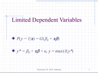
5. For such variables, also known as limited dependent variables, we know the interval that the underlying Y* falls in, but not its exact value Binary & Ordinal regression techniques allow us to estimate the effects of the Xs on the underlying Y*. They can also be used to see how the Xs affect the probability of being in one category of the observed Y as opposed to another.

6. The latent variable model in binary logistic regression can be written as If y* >= 0, y = 1 If y* < 0, y = 0 In logistic regression, the errors are assumed to have a standard logistic distribution. A standard logistic distribution has a mean of 0 and a variance of 2 /3, or about 3.29.

7. Since the residuals are uncorrelated with the Xs, it follows that Notice an important difference between OLS and Logistic Regression. In OLS regression with an observed variable Y, V(Y) is fixed and the explained and unexplained variances change as variables are added to the model. But in logistic regression with an unobserved variable y*, V( y* ) is fixed so the explained variance and total variance change as you add variables to the model. This difference has important implications. Comparisons of coefficients between nested models and across groups do not work the same way in logistic regression as they do in OLS.

8. Comparing Logit and Probit Coefficients across Models

10. x1 and x2 are uncorrelated! So suppressor effects cannot account for the changes in coefficients. Long & Freeses listcoef command can add some insights.

13. Note how the standard deviation of y* fluctuates from one logistic regression to the next; it is about 2.34 in each of the bivariate logistic regressions and 5.34 in the multivariate logistic regression. It is because the variance of y* changes that the coefficients change so much when you go from one model to the next. In effect, the scaling of Y* is different in each model. By way of analogy, if in one OLS regression income was measured in dollars, and in another it was measured in thousands of dollars, the coefficients would be very different.

14. Why does the variance of y* go up? Because it has to. The residual variance is fixed at 3.29, so improvements in model fit result in increases in explained variance which in turn result in increases in total variance. Hence, comparisons of coefficients across nested models can be misleading because the dependent variable is scaled differently in each model.

15. How serious is the problem in practice? Hard to say. We easily found dozens of recent papers that present sequences of nested models. Their numbers are at least a little off, but without re- analyzing the data you cant tell whether their conclusions are seriously distorted as a result. Several attempts of our own using real world data have failed to raise major concerns with the comparisons We asked several authors for copies of their data, but most were unwilling or unable to do so.

16. One author, Ervin (Maliq) Matthew, did graciously provide us with the data used for his paper Effort Optimism in the Classroom: Attitudes of Black and White Students on Education, Social Structure, and Causes of Life Opportunities (Sociology of Education 2011 84:225-245) The paper contains potentially problematic statements such as The effect of race on the dependent variable is even stronger once GPA, SES, and sex are controlled for (Model 2), indicating that when blacks and whites have equal GPAs and family SES, blacks are more likely to agree with this statement. In practice, however, we found that any potential errors were modest, with estimates being only slightly affected by solutions we discuss later. For example, his Table 7 modestly understates how much the effect of race declines as controls are added.

17. Nonetheless, researchers should realize that Increases in the magnitudes of coefficients across models need not reflect suppressor effects Declines in coefficients across models will actually be understated , i.e. you will be understating how much other variables account for the estimated direct effects of the variables in the early models. Distortions are potentially more severe when added variables greatly increase the pseudo R^2 statistics, as the variance of Y* will increase more when that is the case.

18. What are possible solutions? Just dont present the coefficients for each model in the first place. Researchers often present chi-square contrasts to show how they picked their final model and then only present the coefficients for it. Use y-standardization. With y-standardization, instead of fixing the residual variance, you fix the variance of y* at 1. This does not work perfectly, but it does greatly reduce rescaling of coefficients between models. Listcoef gives the y-standardized coefficients in the column labeled bStdy, and they hardly changed at all between the bivariate and multivariate models (.3158 and .2095 in the bivariate models, .3353 and .2198 in the multivariate model).

19. The Karlson/Holm/Breen (KHB) method (Papers are available or forthcoming in both Sociological Methodology and Stata Journal) shows promise According to KHB, their method separates changes in coefficients due to rescaling from true changes in coefficients that result from adding more variables to the model (and does a better job of doing so than y-standardization and other alternatives) They further claim that with their method the total effect of a variable can be decomposed into its direct effect and its indirect effect.

20. We would add that, when authors estimate sequences of models, it is often because they want to see how the effects of variables like race decline (or increase) after other variables are controlled for. The KHB method provides a parsimonious and more accurate way of depicting such changes. Well first present a simple example showing the relationship between diabetes, race & weight.

21. khb example 1

22. Possible interpretation of results In the line labeled Reduced, only black is in the model. .6038 is the total effect of black. However, blacks may have higher rates of diabetes both because of a direct effect of race on diabetes, and because of an indirect effect: blacks tend to be heavier than whites, and heavier people have higher rates of diabetes. Hence, the line labeled Full gives the direct effect of race (.5387) while the line labeled Diff gives the indirect effect (.065)

23. Khb Example 2 Matthew (2011; see Table 7, p. 240) examines the determinants of how likely a student is to feel they will have a job he or she enjoys (0 = 50 percent or lower; 1 = better than 50 percent). In the first model, race (0 = white, 1 = black) is the only independent variable. The estimated effect of race is -.510. In the final model controls are added for GPA, SES, and others. The effect of race declines to -.471, an apparent -.039 drop. The khb method shows that the decline is actually about twice as large. Again this is at least partly because the variance of y* becomes greater as more variables are added, causing coefficients to increase.

25. Selected References Karlson, Kristian B., Anders Holm and Richard Breen. 2011. Comparing Regression Coefficients between Same-Sample Nested Models using Logit and Probit: A New Method. Forthcoming in Sociological Methodology . Kohler, Ulrich, Kristian B. Carlson and Anders Holm. 2011. Comparing Coefficients of nested nonlinear probability models. Forthcoming in The Stata Journal . Long, J. Scott and Jeremy Freese. 2006. Regression Models for Categorical Dependent Variables Using Stata , 2nd Edition. College Station, Texas: Stata Press.